Harmonic solutions of propagation equations

The solutions of the propagation equation are either scalar or vector functions. They must reproduce the same function “farther on” and at a “later time.” In order to be a solution of the equation, the function depends on the coordinate : .

Generally, for waves that propagate towards positive the harmonic solutions are written as follows:

where is the wave vector :

and represents the vector with unit length that describes the direction of the wave propagation , is the wavelength in vacuum, and the wavelength in the medium. Similarly, for waves that propagate towards negative , the harmonic solutions are written as:

In the case of plane and monochromatic waves, the propagation is rectilinear; taking z for example, the propagation equation in vacuum would be written as:

and the solution that propagates towards positive z would be:

The wave surface, which is associated with the propagation is given by equiphase planes such that:

and it is perpendicular to the wave vector .

In the case of spherical waves, the propagation has a spherical symmetry, and the solution which propagates towards positive is:

In this case, the component of the field depends only on r with a coordinate system centered on the point of convergence (or divergence). If the wave is divergent, this is a source point; if the wave is convergent, then it is a focalization point.

The equiphase surface that describes the wave surface is a sphere centered on the source point. A divergent wave is written:

and a convergent wave:

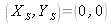
It is helpful to expand the formalism in the case of a cartesian coordinate system. In figure 1, the source is situated at a point in the coodinate plane and the wave propagates by following the positives z.

We can see that:

The wavefront that propagates in the plane situated at the distance from the source is written as [1]:

This expression is not easy to use. In order to reduce the complexity of writing in cartesian coordinates, we use approximations for the distance between the source and the observed wavefront.  These approximations are based on the development of the square root in the exponential function [1]. Indeed, if , we have:

and if we only use the first two terms of the development, we have:

For the denominator, we use a first order approximation:

Thus, from now on, the wavefront that propagates in the plane situated at distance from the source is written:

The validity of this approximation is determined by the errors caused when the higher order terms of the development can no longer be neglected. A satisfactory condition would be that the maximum phase variation caused by a2/8 generates a phase variation much lower than 1 radian. The reader can verify that the condition for validity is the following [1]:

In order to assign the order of magnitude, let us consider a source situated at and a square observation region of 50mm on its side, the wavelength being equal to 0.5 μm, we determine that .