Discrete bidimensional systems

The results regarding bidimensional filtering can be easily transposed to the domain of discrete signals. Most filters that are currently applied to these images are both linear and invariant with spatial translations. In this section, we will study in great details the mechanism of the convolution operation in the case where it is applied in the spatial domain (by opposition to the frequency domain).

A discrete bidimensional system S is defined by an operator which establishes a correspondence between two sets of bidimensional signals. To each signal x(m,n) is associated a response y(m,n) function of the operator S:

Among the discrete bidimensional systems, a particular class is formed by the systems which are both linear and invariant with spatial translations. We can demonstrate that the input-output relation for such a system is given by an discrete bidimensional convolution operation:

In this relation, h(m,n) is the discrete impulse response of the system. The knowledge of h(m,n) is both necessary and sufficient to fully characterize the system. For the latter relation to make sense, it is necessary that the double sum in k and l is bounded for each signal x(m,n) of bounded amplitude. This condition is realized when the series of terms h(k,l) converges in absolute values. We then talk about a stable system:

The discrete convolution is not the unique method allowing computing the response of a discrete bidimensional system to an excitation. An alternative is given by the finite difference equation which links the inputs and the outputs of a linear and spatially invariant system in various points of the planar spatial domain:

In addition to the knowledge of the coefficients governing the finite difference equation, it is necessary to pre-determine the boundary conditions for the output image y(m,n), i.e. the values taken by the pixels at the border of the domain, where the calculation starts. These conditions are equivalent to the initial conditions defined for monodimensional systems in the temporal domain. It is important to notice that the impulse response does not explicitly appear in the calculation of the output image. This is particularly interesting when it comes to setting up image filters whose response is defined on an unbounded domain. This leads us to distinguish two categories of image filters using the finite difference equation.

Filters of finite impulse response (FIR):

This class of filters corresponds to the particular case where the ensemble of coefficients in the left member of the finite difference equation is reduced to a unique element. The output image pixel y(m,n) is therefore only a function of the input image pixels. There is no recurrence.

One can realize that the impulse response directly appears in the finite difference equation, by noticing that the previous equation is a convolution relation between x(m,n) and the coefficients b(k',l'). Therefore:

Filters of infinite impulse response (IIR):

This is the most general case. Pixel y(m,n) is computed using the pixels of the input image but also using the neighbor pixels of the output image. There is a recurrence relation between the pixels of the output image.

In this case, determining the impulse response is not trivial, and can be done by replacing x(m,n) by a delta function d(m,n) in the finite difference equation, and by specifying the boundary conditions. We can now address the study of the discrete convolution mechanism by restricting ourselves to the FIR filters. In this case, the output image is equal to:

The domain of definition of the impulse response h(m,n) is limited to a matrix of size (K,L). For example, with K=L=3, k1=-1 and l1=-1, we have:

To calculate the output image filtered with h(m,n), we apply a mask to the input image x(m,n) which extracts the region involved in the calculation of pixel y(m,n), in accordance with the previous relation. The full image calculation is made by iteratively shifting the mask on all the pixels of image x(m,n). When the mask is placed on regions encompassing pixels falling outside of the image, those pixels are set to zero. The following example shows how this mechanism works.

We consider an input image A(m,n) and a filter h(m,n) such that,

B(m,n) is the output image. The first step consists in building a mask g(m,n) starting from the filter. Indeed, equation (5.8) brings into play the elements h(m-l,n-k) of the filter impulse response, resulting from a reversal of h(l,k) combined with a translation of parameters (m,n):

The second step consists in implementing two nested loops on matrix A in order to cover all pixels. Operation (5.8) is computed at each iteration. The figure below shows how matrix A and mask g are positioned for the first iteration:

Figure 5-1: Illustration showing how image A et mask g are positioned for the filtering first iteration. [zoom...]

This first iteration allows calculating pixel (1,1) of image B. Its value is given by:

The pixels of image A can be scanned in any order. We made an arbitrary choice here, but we could have equally started by positioning the mask on the central pixel of matrix A. The full calculation gives the following matrix B(m,n):

Examples of filters FIR

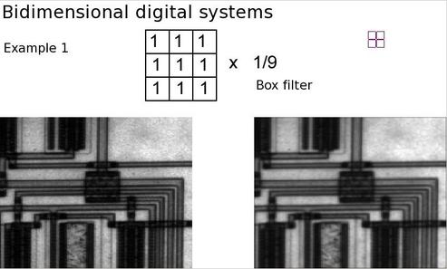
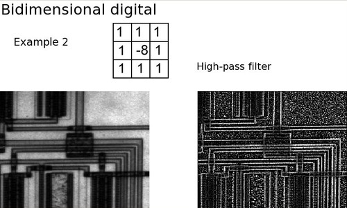
Before closing this chapter, we will review a few examples of FIR filters widely used in image processing. The following examples illustrate the results obtained when filtering a gray-level image reproducing the picture of a printed circuit board. This image mainly shows an network of horizontal and vertical lines corresponding to the current ducts.

Simple averaging filter (box filter)

This filter is defined by a rectangular function, which is normalized so that the gain is equal to 0 dB at the origin of the frequency space. The impulse response of the 3x3 filter reads:

Figure 5-2 : Applying a box filter to the test image. [zoom...]

Such a filtering results in smoothing the discontinuities visible on the printed circuit board. The circuit lines thus look blurred. We can notice that this phenomenon is independent from the image orientation. In the frequency domain, the average filter is a low-pass filter.

High-pass filter

Here is the impulse response of a simple 3x3 high-pass filter:

Figure 5-3: Application du filtre passe-haut sur l'image test. [zoom...]

This filter highlights the discontinuities of the image, and therefore we observe a strengthening of the circuit layout. We also notice a higher level of noise, which can be observed in particular in the uniform regions outside of the circuit lines.

The vertical differential filter

The 3x3 vertical differential filter has an impulse response equal to:

Figure 5-4: Applying the vertical differential filter to the test image [zoom...]

We clearly notice on the filtered image that only the contours of the vertical lines are highlighted. The horizontal lines have disappeared because their contours have been smoothed by an averaging effect on the vertical direction.

AccueilOutils transversesNouvelle pageInformations sur le cours (ouvrir dans une nouvelle fenêtre)Sampling and quantizationConclusion