Examples

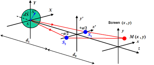
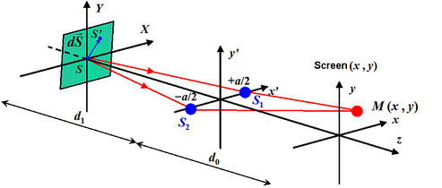
Let us examine the decrease in contrast produced by an extended source with a circular shape that is emitting a monochromatic radiation of . Figure 16 shows the notations. We note 2R the diameter of the source.

The circular source has a uniform brightness that can be described by the following function:

The Fourier transform of the source's angular distribution is given by:

The source has a circular symmetry; we can use a transformation in polar coordinates for (X , Y) and , i.e.:

thus,

or also:

considering that:

J0 being the Bessel function of the first kind of order 0, we have:

Due to the definition of the brightness function, it follows that:

Assuming , we obtain:

along with the equality:

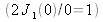
J1 being the Bessel function of order 1 such that , we finally obtain:

Since we have (figure 16):

the degree of spatial coherence of the circular source is finally written as :

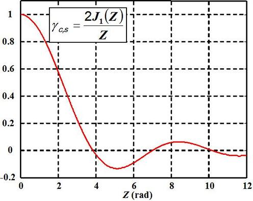
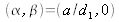
The formula for the degree of spatial coherence of the circular source is where 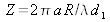. Figure 17 shows the outline of the degree of spatial coherence of the circular source as a function of the value of Z expressed in radians.

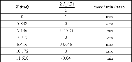
Table 2 gives the values of Z for maxima, minima, and zeros of the degree of coherence.

The zeroes of the degree of spatial coherence are not equidistant. The first contrast cancellation is obtained by:

i.e. by a distance between the secondary sources that is equal to:

Remember that 2R represents the source diameter.

As a result of the angular diameter from which the source is seen from the plane of the secondary sources, we obtain:

As a numerical example, let us consider the case of the Sun for which the apparent angle of observation from Earth is 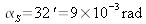. The preceding relation gives for . If we want to observe contrasted interferences at a point M on the screen, the secondary sources must not be separated by a distance greater than this value. Sunlight, therefore, has a weak spatial coherence.

For secondary sources of the same amplitude, the interference signal at a point M on the screen can be written as:

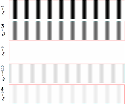
Figure 18 shows the interferograms obtained for the different values of the degree of coherence on a screen.

The fringe contrast evolves as a result of the source radius R following the curve in figure 17. If the value of R is low, the fringe contrast is ostensibly equal to the unit. As R increases, the contrast diminishes and eventually becomes null when . Then, when the contrast becomes nevative, the bright fringes occupy the position of the dark fringes and vice versa; this inversion can be observed quite easily in figure 18, even if the contrast is rather weak . If the value of R continues to increase, the fringes become less and less visible until they disappear completely.

Now let us examine the decrease in contrast caused by an extended source with a rectangular shape. Figure 19 shows the notations. We note as the dimensions of the source.

The circular source has a uniform luminance that can be described by the following function:

The Fourier transform of the light distribution of the source is given by:

Keeping in mind the definition of the brightness function, we have:

This expression can be easily integrated, so we find that:

Since the secondary sources are reduced to two points, , we have:

For the case illustrated in figure 19, the degree of spatial coherence of the rectangular source is written as:

The degree of spatial coherence of a rectangular source has the shape of a sinc function. Figure 20 shows the shape of the degree of spatial coherence of the rectangular source as a function of the value of Z expressed in radians.

The zeroes of the degree of coherence are equidistant. The contrast is cancelled at:

The first zero is obtained for the distance between the secondary sources that is equal to:

This expression gives us an estimate of the width of the spatial coherence of the source.